The Trials and Tribulations of Optimization

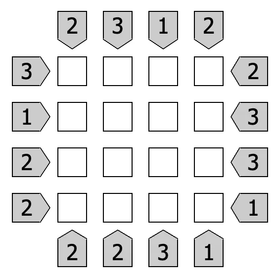
This year, while others were passing the time during the summer slump by playing Sudoku, I was practicing the Skyscraper Game. An N x N grid, with buildings ranging in height from 1 to N, each height appearing exactly once per row and per column. On the sides, as clues, the number of buildings an observer would see when looking into the grid.

And since in August the whole of France comes to a standstill and the afternoons stretch on endlessly, I decided to implement an algorithm capable of solving any puzzle in this game on its own. Many hours later, here is the result (https://github.com/mathieueveillard/skyscrapers) and a few thoughts on optimization.

Yep… The game, which seems easy at first glance, gets seriously tricky as the grid gets bigger and clues become scarcer. This one, a 5x5 grid, is already significantly more complicated.

If you get hooked on the game and feel like looking for an algorithm, you’ll quickly discover that it’s a constraint programming problem, with the constraints being:

• Side views
• The heights of the buildings pre-positioned on the grid

No premature optimization?

Everyone knows Donald Knuth’s warning. However, it should not be understood as an invitation to write completely naive algorithms that ignore a difficulty known from the outset.

The naive algorithm here would be to generate all possible grids and then eliminate those that don’t satisfy all the constraints. Considering the N possible heights for each of the N² buildings, that makes N^(N²) grids of N² values… Let’s just forget about it.

No, we need to flip the problem and generate the “candidate” rows and columns based on the constraints we have. The idea is therefore to start with a sequence [1, 2, …, N] corresponding to a view of N (left-hand view). Moving any building to the right reduces the view by 1.

Example, on a 4x4 grid:

[1, 2, 3, 4] -> view = 4
Move the 1: [2, 1, 3, 4] or [2, 3, 1, 4] or [2, 3, 4, 1] -> view = 3
Move the 2: [1, 3, 2, 4] or [1, 3, 4, 2] -> view = 3
Move the 3: [1, 2, 4, 3] -> view = 3

Ideally, only one candidate is valid once placed in the grid. But in most cases, several candidates are valid, and you’ll have to make an assumption each time, which you’ll later validate or invalidate (completed grid vs. dead end a few rows or columns down). It’s therefore a backtracking algorithm that recursively explores a tree of possibilities.

And in the “let’s avoid doing anything too gross” department, memoization is your friend 😊

Ah, Pareto…

As always, 20% of the time you spend on the problem will yield 80% of the optimization benefits, while you’ll be sweating it out for the remaining 80% of the time to reach 100% optimization (assuming, of course, that it can ever be achieved). Ouch.

Here are the two main areas of focus:

• Work on the most constrained rows/columns first (generally, two views are better than one and especially better than zero, and a high view is better than a low one);

• Generate candidates more efficiently for rows/columns without a view indication (e.g., 1 _ _ 5 3 offers only two possibilities, which are easily identifiable).

All in all, the optimization reduced the runtime by a factor of 50, but a 7x7 grid still takes about 20 seconds to solve, and I wouldn’t dare estimate the time complexity of the algorithm 🥲

Into the Unknown

Optimizing an algorithm means venturing into uncharted territory: when you set out to implement an improvement, you generally can’t quantify the expected benefit in advance, all the more so because the search tree depends on the input data. Expect to sometimes work for a long time for results that are barely noticeable.

And that will serve as my conclusion.